This Technical Note summarizes the current state of understanding of various issues involved into design of the L1 Database use by the Alert Production pipeline. This is not a final document and will likely be updated when more information becomes available. This initial revision is compiled from information in JIRA tickets DM-5316, DM-5509, and DM-5545.
The following sections cover various aspects of the design in no particular order.
L1 database schema
The schema of the L1 database is outlined in DPDD (LSE-163). There are three tables which contain most of the data of the L1 database – DiaSource, DiaForcedSource, and DiaObject. Here are the approximate sizes in bytes of the rows in those tables as given in the Sizing Model Spreadsheet (LDM-141) and estimated from DPDD:
| Row size, bytes | ||
|---|---|---|
| Table name | LDM-141 | DPDD |
| DiaObject | 1,124 | 1,536 |
| DiaSource | 333 | 232 |
| DiaForcedSource | 41 | 33 |
| SSObject | 488 | 424 |
There is some discrepancy between the two sets of numbers; calculations below use estimates from LDM-141.
Current baseline assumptions
The baseline design of L1 is explained in LDM-135 and it is based on input from DPDD and figures from the Sizing Model Spreadsheet (LDM-141). The current baseline design assumes that L1 database is replaced every year by an improved version produced by DRP as a part of the Data Release. It is expected that L1 data from each Data Release does not contain the full history of DiaObject but only the most recent version of it, while still keeping full set of DiaSource and DiaForcedSource tables. Because DiaObject has the largest record size, resetting DiaObject after each DR helps to control the size of the DiaObject table.
Figure 1 shows an estimated behavior of the count of the rows in three largest tables from the L1 databases, based on the above assumptions. Figure 2 shows the sizes of the corresponding tables calculated for the numbers of rows. Calculated sizes are based on the row sizes as defined in LDM-141, which do not quite agree with DPDD-defined schema and will likely need some adjustment. Also these sizes do not take into account overhead due to data organization and indexing which can be significant.
In the current baseline design the total size of the tree major tables will likely reach and exceed 100TB mark per single L1 database replica.
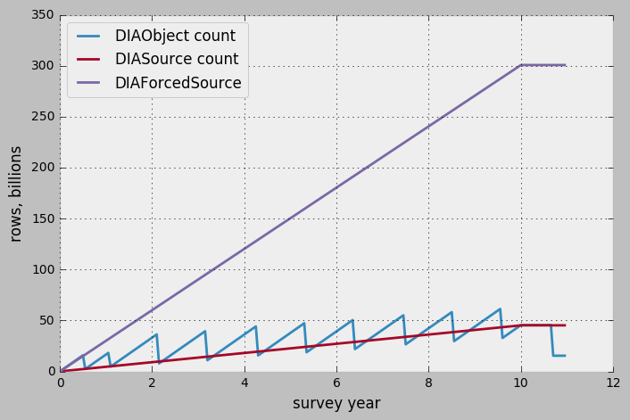
Figure 1 Estimate of the row count in L1 database for three major tables.

Figure 2 Estimate of the table sizes in L1 database for three major tables.
Revised L1 database design
L1 database switch-over after each DRP is seen as too disruptive for the scientific community, so a new approach was proposed by the Science Pipelines Definition Working Group. In this proposal there is no annual switch-over to DRP-produced L1 tables; instead, the L1 database continues to accumulate its data indefinitely. This means that the entire history of DiaObject is kept forever, which increases significantly the row count and size of the DiaObject table.
Figure 3 shows the estimated row count for the same major tables in the new proposal (DiaSource and DiaForcedSource counts do not change). Figure 4 shows the sizes of the corresponding tables.
In this new proposal the total size is dominated by the DiaObject table, and could reach 400TB (without accounting for overhead of indexing and storage).
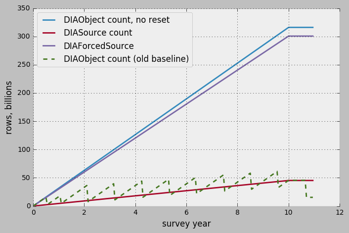
Figure 3 Estimate of the row count in L1 database in new proposal, baseline estimate of the DiaObject is given for comparison.
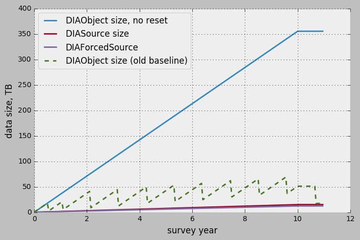
Figure 4 Estimate of the table sizes in L1 database in new proposal, baseline estimate of the DiaObject is given for comparison.
Queries on the L1 database
The most important client of the L1 database is the Alert Production (AP) pipeline, so the the L1 database will be optimized for queries generated by AP. AP will need following data from the L1 database for its operation on a single visit:
- The most recent version of all DIAObjects in the region covered by a CCD (this may be limited to DIAObjects produced in last 12 months)
- The last 12 months of DIASources from the same region, matching the DIAObjects selected above
- History of DIAForcedSources from the same region, again the same 12 months and matching selected DIAObjects
AP will produce more data to be stored in the L1 database for each visit:
- a set of DIASources discovered in a visit
- a set of DIAObjects, either new or updated versions; for new objects also store associations to L2 Objects.
- a set of DIAForcedSources for forced measurements (DIAForcedSources will also be produced in precovery processing which happens during the day)
The queries to retrieve the data have both spatial and temporal constraints. Given the baseline schema (LDM-135) for the DIAObject table which includes a validity interval, the above requirements translate into the following set of queries:
- Select all most recent versions of DIAObjects for a specified region, optionally limited to records not older than 12 months. The region may cover either a single CCD or the whole camera, depending on how Source-to-Object matching is performed.
- Select the elements of the DIASource and DIAForcedSource history for the last 12 months which match the set of DIAObjects selected in previous query. It may be more efficient to select based on the region, and then filter unmatched sources on the client side.
- Insert a new set of DIAObjects, which may also update the validity interval of the latest version of any corresponding object already stored in the database.
- For new DIAObjects, store associations of the DIAobject to L2 Objects.
- Insert a new set of DIASource and DIAForcedSource records.
Visit data dependency
There will be spatial overlaps between consecutive visits, and there may be multiple consecutive visits of the same region. This causes data dependency between jobs processing these consecutive visits, because each job will require a set of the most recent DIAObjects which may overlap with the set of the DIAObjects produced in the previous visit. This argument applies to DIASources and DIAForcedSources as well.
There are significant implications of this dependency for the L1 database access pattern. Without this data dependency it would be possible to start pre-loading all of the necessary L1 data as soon as pointing coordinates become available (typically right before first exposure). With the data dependency the data can still be pre-loaded, but some of that data may need to be updated when the processing of the previous visit finishes (typically a minute or less after the second exposure).
Solving this problem may require additional synchronization and/or data exchange between jobs processing different visits. Alternatively, all processing that needs L1 data (source association and alert production) could be moved to a separate processing to be done sequentially with the results from one visit being immediately available to next visit, though this may severely limit parallelism.
Partitioning
It is clear that the volume of data in L1 database will be extremely large. Updating and indexing data volumes of that scale needs special care for scalability issues. One standard tool to keep these issues under control is horizontal partitioning of large tables. In the case of the L1 database, partitioning can be done based on time ranges with a range length related to typical time periods of typical queries (e.g. 12 months or shorter). With that approach only the latest shards will be update-able and queries will typically only use limited number of recent shards.
Partitioning introduces additional complications for operations: new partitions need to be created regularly, and data access requires writing queries involving one or more shards. There may be additional complications for the DiaObject table whose, records represent time intervals which potentially can span more than one shard.
In addition to regular partitioning, it may be reasonable to create specialized partitions or views that contain data relevant for some specific queries (e.g. query for most recent versions of DiaObjects). These views will result in duplication of some information from the regular database which will require special care to guarantee data consistency.
Indexing and Locality
All of the most important queries from the list above require geometry-based
selection of a small patch of the sky, typically a single CCD or the
entire region of a single visit. It is extremely important to serve these
sorts of queries in the most efficient way. One possible approach for fast
access is to use spatial indexing optimized for spherical geometry. There
may be several candidates for this sort of indexing scheme such as
Hierarchical Triangular Mesh (HTM) or Quad Tree Cube (Q3C). Both of these
indexing strategies map small sky regions to a set of integer numbers, and for both
of them mapping of CCD regions to index ranges can be performed on the client
side without special support on the database server side. These two indexing
schemes will be implemented in LSST package sphgeom.
In addition to spatial indexing, other indices may be important. For example, selection of the most recent DiaObject version could possibly be achieved via a special index on DiaObject validity interval. This may create additional overhead in both space and CPU time. Specialized structures could be used in some cases, e.g. the previously mentioned special partitions with a subset of the data.
Typical queries will return a large number of records, and this may translate into a large number of I/O operations for the database server. To reduce the number of disk seeks and the resulting latency it will be important to think about data locality and try to keep related data physically close on disk. How exactly this can be controlled depends on the particular database technology used, e.g. the MySQL InnoDB engine orders data according the primary index, and MyISAM table format stores records in order of insertion. Some storage technologies (SSD) can help to avoid the issue by reducing seek time, though exact gain is hard to predict. Extensive prototyping at large scale will be needed to understand and evaluate possible approaches.
Replication and fail-over
The L1 database needs a high-availability solution with a reasonably short downtime in case of fail-over. Additionally, a read-only instance of the L1 database will be deployed at the base site and it will need to be updated continuously from the master copy with a reasonably short delay.
Arguably the simplest architecture to satisfy these requirements consists of two instances at the main site with master-master replication between them, and a slave instance at base site with master-slave replication from the main site. Master-master replication allows quick fail-over in case of a master failure; this fail-over does not need re-configuration of the server instances and happens entirely on the client site. Currently the MySQL C API does not support transparent fail-over, but it can be implemented in higher-level API or with the help of a separate proxy layer. Master-slave replication only supports single masters; in cases of master failure it will need manual intervention to switch to a different master instance.
In addition to a basic MySQL replication solution there are other third-party replication solutions (e.g. MariaDB Galera Cluster) which could be used for the same purpose. PostgreSQL also supports master-master and master-slave replication mechanisms, and could be used in a similar architectural approach.
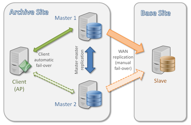
Figure 5 Anticipated architecture for L1 replication.